Visualization
Visualization of Simplicial Complexes and Generators
In this section, we’ll visualize simplicial complexes using plotly.
import numpy as np
import bats
from bats.visualization.plotly import ScatterVisualization
import scipy.spatial.distance as distance

np.random.seed(0)
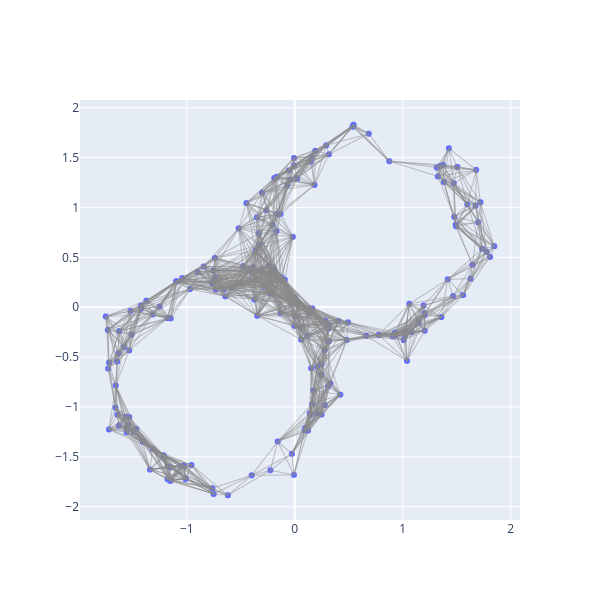
Let’s generate a figure-8 as a data set.
def gen_fig_8(n, r=1.0, sigma=0.1):
    X = np.random.randn(n,2)
    X = r * X / np.linalg.norm(X, axis=1).reshape(-1,1)
    X += sigma*np.random.randn(n, 2) + np.random.choice([-1/np.sqrt(2),1/np.sqrt(2)], size=(n,1))
    return X

n = 200
X = gen_fig_8(n)
First, we’ll construct a Rips complex on the data.
pdist = distance.squareform(distance.pdist(X, 'euclidean'))

R = bats.RipsComplex(bats.Matrix(pdist), 0.5, 2)
fig = ScatterVisualization(R, pos=X)
fig.update_layout(width=600, height=600, showlegend=False)
fig.show()
A ScatterVisualization object inherits from a plotly Figure, so you can add additional traces, update layout, or call any methods you’d like.
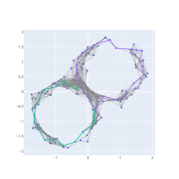
Now, let’s visualize generators
fig.show_generators(1)
fig.show()
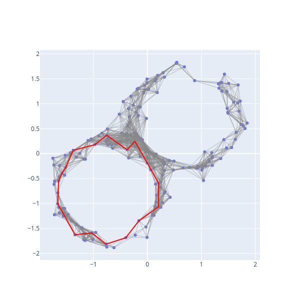
Let’s now look at a single generator:
fig.reset() # resets figure to have no generators
fig.show_generator(0, hdim=1, color='red')
fig.show()
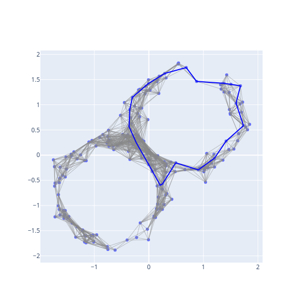
Let’s visualize the second generator by passing in the representative 1-chain:
RC = bats.ReducedChainComplex(R, bats.F2())
r = RC.get_preferred_representative(1, 1)
fig.reset()
fig.show_chain(r, color='blue')
fig.show()
Visualization of Maps
You can visualize a SimplicialMap with a MapVisualization.
import numpy as np
import bats
from bats.visualization.plotly import MapVisualization
import scipy.spatial.distance as distance

np.random.seed(0)
Let’s generate a cylinder in three dimensions:
def gen_cylinder(n, r=1.0, sigma=0.1):
    X = np.random.randn(n,2)
    X = r * X / np.linalg.norm(X, axis=1).reshape(-1,1)
    X = np.hstack((X, r*np.random.rand(n,1) - r/2))
    return X

X = gen_cylinder(500)
We’ll generate a Rips Complex with parameter 0.25
pdist = distance.squareform(distance.pdist(X, 'euclidean'))
R = bats.RipsComplex(bats.Matrix(pdist), 0.25, 2)
Let’s investigate the inclusion of the lower half of the cylinder
inds = np.where(X[:,2] < 0)[0]
Xi = X[inds]
pdisti = distance.squareform(distance.pdist(Xi, 'euclidean'))
Ri = bats.RipsComplex(bats.Matrix(pdisti), 0.25, 2)
The inclusion map is
M = bats.SimplicialMap(Ri, R, inds)
Now, we can construct a visualization
fig = MapVisualization(pos=(Xi,X), cpx=(Ri,R), maps=(M,))
fig.update_layout(scene_aspectmode='manual',
                  scene_aspectratio=dict(x=1, y=1, z=0.5))
fig.show()
The show_generator method will visualize homology generators in the domain by visualizing the preferred representative used in calculations. By default, the image of the chain is visualized in the range, as well as the preferred representative for the homology class.
fig.reset()
fig.show_generator(1)
fig.show()
The reset method clears the visualization of chains/generators. You can also change the color of chains and homology. group_suffix can be used to group visualizations in the legend - try using the legend to toggle visualizations below:
fig.reset()
fig.show_generator(5, group_suffix=0)
fig.show_generator(3, color='orange', hcolor='black', group_suffix=1)
fig.show()
Let’s now create a second map from the full data set to a projection onto two coordinates.
Xp = X[:,:2]
pdistp = distance.squareform(distance.pdist(Xp, 'euclidean'))
Rp = bats.RipsComplex(bats.Matrix(pdistp), 0.25, 2)
M2 = bats.SimplicialMap(R, Rp) # inclusion map
We can visualize the three spaces, with the maps between them, and mix 2-dimensional and 3-dimensional visualizations. Note that the homology class visualized in show_generator(1) is killed by the second map.
fig = MapVisualization(pos=(Xi,X, Xp), cpx=(Ri,R,Rp), maps=(M,M2))
fig.update_layout(scene_aspectmode='manual',
                  scene_aspectratio=dict(x=1, y=1, z=0.5))
fig.show_generator(1, color='green', hcolor='black', group_suffix=1)
fig.show_generator(5, color='red', hcolor='blue', group_suffix=5)
fig.show()